Introduction to Generative Modeling

This blog provides a primer on generative modeling, summarizing introductory knowledge required before venturing into more advanced topics. It will serve as a foundational piece that I plan to build upon and update whenever necessary. As I delve deeper into the subject, I intend to create more comprehensive articles focusing on various topics, This blog acts as an initial stepping stone towards that goal.

Motivation

Generative modeling, promotes understanding of causual relationships between variables involved as we try to understand how their values culminate to generate a certain outcome. By mimicking the underlying generative process, this approach allows us to not only replicate outcomes but also unravel the interplay between variables involved and their influences.

Following is a paragraph from “An Introduction to Variational Autoencoders” [1].

“A generative model simulates how the data is generated in the real world. “Modeling” is understood in almost every science as unveiling this generating process by hypothesizing theories and testing these theories through observations. For instance, when meteorologists model the weather they use highly complex partial differential equations to express the underlying physics of the weather. Or when an astronomer models the formation of galaxies s/he encodes in his/her equations of motion the physical laws under which stellar bodies interact. The same is true for biologists, chemists, economists and so on. Modeling in the sciences is in fact almost always generative modeling”.

From a probablistic viewpoint, data is generated by an underlying distribution $p_{data}$. Generative modeling requires us to model the distribution of the data $p_{\theta}$. This empowers us with the ability to deduce the probability of a specific dataset occurrence and, of even greater significance, provides a means to draw samples effectively generating outcomes adhering to the characteristics of the data distribution.

Problems we would like to solve using generative models

• Data Generation : Synthesizing image, video, speech, text and more.

• Data Compression and meaningful representation : In a generative process, the data is assumed to be generated in a hirerachy, first concepts are generated in a concept (latent) space. Data compression and meaningful representations revolve around the idea of creating efficient mappings between the real and the latent space.

• Anomaly Detection : It is done through either likelyhood estimatation or reconstruction error.

Probablistic modeling

The generative model is parameterised by $p_{\theta}$. Our objective then becomes to minimize the “distance” between $p_{data}$ and $p_{\theta}$.

While various concepts of distances are present, the Kullback-Leibler ($D_{KL}$) divergence stands out as a widely embraced measure. It is formally given by the following equation.

Subsequently, we will explore alternate distance metrics in use. A rationale supporting its prominence stems from the requirement that approximating KL divergence involves sampling from the data distribution.

Let $D = \lbrace x^{(1)},x^{(2)},…x^{(n)} \rbrace$ be an i.i.d dataset sampled from $p_{data}$. Then the $D_{KL}$ between the distibutions could be approximated as:

This is useful because, in order to optimize $\theta$, we could remove the numerator term.

$ \theta^{*} = argmin_{\theta} \frac{1}{n} \sum_{i=1}^{n} \log \left( \frac{p(x^{(i)})}{p_{\theta}(x^{(i)})} \right) $

$ \Rightarrow \theta^{*} = argmin_{\theta} \frac{1}{n} \sum_{i=1}^{n} \log \left( \frac{p(x^{(i)})}{p_{\theta}(x^{(i)})} \right)$

$ \Rightarrow \theta^{*} = argmin_{\theta}\sum_{i=1}^{n} \log ( p(x^{(i)})) - \sum_{i=1}^{n}log({p_{\theta}(x^{(i)})}) $

$ \Rightarrow \theta^{*} = argmax_{\theta}
\sum_{i=1}^{n}log({p_{\theta}(x^{(i)})}) $

Hence, minimizing KLD is same as maximizing likleyhood of the sampled dataset given the parameters$\theta$.We used a sample mean to approximate the expectation, and this type of estimation is also referred to as Monte Carlo estimation. We will revisit Monte Carlo estimates at a later point. For now, let’s delve deeper into the analysis of the KL divergence.

Asymmetric nature of the KL divergence

The asymmetric nature of the Kullback-Leibler (KL) divergence is a fundamental characteristic that distinguishes it from other distance metrics. KL divergence measures the difference between two probability distributions (P) and (Q) in a non-symmetric manner.

This asymmetry is evident in the formula for KL divergence:

We find it convinient for measuring the divergence as $D_{\text{KL}}(p_{data} | p_{\theta})$. This way we don’t need to explicitly know the distribution $p_data$ that we trying to model. But, for a while lets focus on what the different ordering entails. Lets take a look at an illustration given in “NIPS 2016 Tutorial:Generative Adversarial Networks” [2].

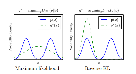
Before making any remarks, it is important to understand the context of the image presented. The data distribution shown in blue (p) is bi-modal, whereas the capacity of the model distribution shown in green is limited to be an univariate gaussian. The distribution of q is limited, just as our model would be limited in terms of the actual complexity of any real data that we are trying to learn. As summarized by Goodfellow [2] :

“We can think of $D_{KL}(p_{data} | p_{model})$ as preferring to place high probability everywhere that the data occurs, and $D_{KL}(p_{model} | p_{data})$ as preferrring to place low probability where data doesnt occur.”

Looking at it from a sampling standpoint, an argument could be made in favor of utilizing KL in the opposite direction. This is because it ensures the generation of samples that appear realistic, but there’s a risk that these samples might only originate from a specific mode within the distribution, a phenomenon known as “mode collapse.” This approach might not be effective in generating data that covers a wide range of high-density regions.

Efficacy of a generative model

We will see later on the different ways to design generative models. We can ask three core questions for assessing the efficacy of such models:

1. $\textbf{Density Estimation}$: When presented with a specific datapoint $x$, what probability density function value $p_{\theta}(x)$ is attributed to it by the model ?

2. $\textbf{Sampling}$: How can we generate fresh, previously unseen data points from the model distribution, represented as $x_{\text{new}} \sim p_{\theta}(x)$?

3. $\textbf{Unsupervised Representation Learning}$ : There are some models such as Variational autoencoders (VAEs) which assumes a hierachical data generation process, where first some latent variable (repesentation) is generated and then the data is generated by conditioning on it. From such models, we would like to uncover significant feature representations for a given datapoint $x$. How do we acquire meaningful features that capture the essence of $x$ in an unsupervised manner? Such models bridge a connection between representation learning and generative modeling.

Simple parametric model

Simplest example that I could think of is of a univariate gaussian distribution. It has two parameters mean $\mu$ and variance $\sigma^2$. Denoted by $x \sim N( x ;\mu,\sigma^2)$. Then the probability density is given as follows:

Assume we have a dataset of independent samples $\lbrace x_1, x_2, \ldots, x_n \rbrace$ from the Gaussian distribution. The likelihood function is:

The log-likelihood function is: \(\log L(\mu, \sigma | x_1, x_2, \ldots, x_n) = -\frac{n}{2} \log(2\pi\sigma^2) - \frac{1}{2\sigma^2} \sum_{i=1}^{n} (x_i - \mu)^2\)

The maximum likelihood estimate for $\mu$ is obtained by differentiating the log-likelihood with respect to $\mu$ and setting it to zero: \(\frac{\partial}{\partial \mu} \log L = \frac{1}{\sigma^2} \sum_{i=1}^{n} (x_i - \mu) = 0\) Solving for $\mu$: \(\hat{\mu} = \frac{1}{n} \sum_{i=1}^{n} x_i\)

The maximum likelihood estimate for $\sigma^2$ is obtained by differentiating the log-likelihood with respect to $\sigma^2$ and setting it to zero: \(\frac{\partial}{\partial (\sigma^2)} \log L = -\frac{n}{2\sigma^2} + \frac{1}{2(\sigma^2)^2} \sum_{i=1}^{n} (x_i - \mu)^2 = 0\) Solving for $\sigma^2$: \(\hat{\sigma^2} = \frac{1}{n} \sum_{i=1}^{n} (x_i - \mu)^2\)

As we can see, in situations involving a straightforward parametric model, it’s easy to perform the parameter optimization by maximizing the likelihood of the training data. Nevertheless, circumstances don’t always permit us to observe all the variables. Consequently, when dealing with more sophisticated latent variable models, we may need to employ alternative methods like the EM-Algorithm or Variational Inference which I will discuss in a seperate blog.

Equipping with some useful concepts

I would like to finish this blog with some useful concepts which would come in handy in our future discussions.

1. Probabilistic chain rule

This rule allows us to break down complex joint probabilities into a sequence of conditional probabilities.It plays a crucial role in autoregressive generative model. In autoregressive models, the idea is to predict the value of a variable at a specific time point based on its previous values.

2. Monte-carlo methods

The expectations of any function of a random variable could be calulated simply by knowing the probability distribution of the random variable involved. This is also known as the law of the unconscious statistitian (LOTUS).

Let $x \sim p(x)$ and $z= f(x)$. Then $E_{p(z)}[z]$ is given as:

Our goal is to solve this integral, typically solving the integral becomes very challenging and practically remains intractable. Most of the time, we would find that it is easier to estimate the value of expectation by performing certain operations on samples generated from known distributions. Such techniques are known as monte-carlo methods.

One of the fundamental techniques involves sampling from the probability distribution p(x). With this method, one can estimate the expected value by simply calculating the average of the function’s values obtained from the generated samples.

We could easily see that this quantity is an unbiased estiamtor (i.e., $E[S_n] = E[f(x)] $). And $Var(S_n) = \frac{1}{n} var(f(x))$. As n $ \rightarrow \infty $, variance of the estimator is zero.

In Monte Carlo estimation, the central question typically revolves around determining the number of samples required to obtain a reasonable estimate. More sohisticated techniques will result is a faster decay of variance. There are instances where sampling from the distribution p is not straightforward, and in such scenarios, importance sampling is often employed.

The idea is simple, instead of sampling from p (which may be impossible), a known distribution q is used.

Where $ w(x) = \frac{p(x)}{q(x)}$ is also known as the importance weight.

The variance of the estimator is influenced by the selection of the probability density function $q$. It can be demonstrated that when $q(x)$ is equal to the ratio of $p(x)$ multiplied by $f(x)$ (i.e., $q(x) = p(x)\vert f(x) \vert /E_p[f(x)]$), then the variance becomes zero.

3. Gradient of expectation

In many situations, while perfroming gradient decsent, we often come across taking a gradient over a loss which constitutes an expectation term. Since, most of the time the intergal calculation is not tractable, we resort to sampling as an approximation. Recalling Lebniz rule from multivariate calculus course, if $ F(\theta) $ is defined by the integral: \(F(\theta) = \int_{a(\theta)}^{b(\theta)} f(x, \theta) \, dx\)

Then derivative of $F$ with respect to $\theta$ is given by: \(\frac{d}{d\theta} F(\theta) = \int_{a(\theta)}^{b(\theta)} \frac{\partial}{\partial \theta} f(x, \theta) \, dx + f(b(\theta), \theta) \cdot b'(\theta) - f(a(\theta), \theta) \cdot a'(\theta)\)

For our purpose, let F be $E_{x \sim p_\theta}[f(x,\phi)]$:

Then calcualting $\nabla_\phi F $ (gradient w.r.t $\phi$ ) is pretty straightforward:

Which could be then approximated by sampling. The more challenging situation is to calcuate $\nabla_\theta F $:

Notice, this time around the gradient is not a distribution anymore, so the integral cant be approximated from sampling from $p$.

There are a lot of tricks in the literature to overcome this challenge [3], for instance, reparameterization is applied in VAE loss calculations. Again, the emphasis of various tricks is upon the convergence of estiamte and ease of calcuation.

One simple trick is to replace the gradient of density with log of density times the density.

Hence the gradient, $\nabla_\theta F $ can be rewritted as,

4.Transforming random variables

Let $F : R^n \rightarrow R^m $ be a diffrentiable transformation (partial derivatives exists).

Then the jacobian of transformation is a matrix defined as: \(J_F = \begin{bmatrix} \nabla^\top F_1(x) \\ \nabla^\top F_2(x) \\ \vdots \\ \nabla^\top F_m(x) \end{bmatrix}\)

Given an invertible transformation $Y =\mathbf{G}(X)​$ the distribution of Y is given by:

And if the jacobian is more convinient to compute in forward direction then:

Invertible transformations are often used context of generative models, such as Variational Autoencoders (VAEs), where they are integral to the reparameterization trick. Also used in Normalizing flows where a seq of invertible transformations are used to directly obtain the distribution of $p(x)$ from the latent variable distribution $p(z)$.

References

1. Kingma, D.P. and Welling, M., 2019. An introduction to variational autoencoders. Foundations and Trends® in Machine Learning, 12(4), pp.307-392.

2. Goodfellow, I., 2016. Nips 2016 tutorial: Generative adversarial networks. arXiv preprint arXiv:1701.00160.

3. Walder, C.J., Roussel, P., Nock, R., Ong, C.S. and Sugiyama, M., 2019. New tricks for estimating gradients of expectations. arXiv preprint arXiv:1901.11311.