Variational Autoencoders
Published:
Note: This blog is not yet complete, and will be updated frequently.
The Latent Variable Model
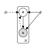
The following generative process is assumed, first sample $z \sim p_\theta(z)$. Then sample x from $p_\theta(x\vert z)$.
The joint distribution for the generative model is given by the Bayes rule.
\[p_\theta(x,y) = p_\theta(z)p_\theta(x|z)\]Likelihood optimization
In order to optimize the parameters of our generative model, we assume that the training set consists of i.i.d observations coming from $p_{data}$. We would then maximize the likelihood of our model. If the marginal $p_\theta(x)$ was tractable then we are done. Unfortunately, this is most of the time not possible.
\[\theta = \arg \max_{\theta} \sum_{i} \log p_\theta(x_i)\]Let’s just concentrate on the expression $log p_\theta (x)$ (i.e., the likelihood of a single example). It simplifies into the following:
\[\log p_\theta(x) = \log \int p_\theta(x,z) dz\] \[= \log \int p_\theta(x|z)p_\theta(z) dz\] \[= \log E_{z \sim p_\theta(z)}[p_\theta(x|z)]\]Estimating the gradient of the expression w.r.t $\theta$ using a Monte Carlo estimation is not straightforward. (But it could be done, using a re-parameterization trick or log-derivative trick etc.) For simplicity, we often assume prior being parameter-free (i.e., $z \sim p(z)$). We can now resort to just taking the average of $p_\theta(x\vert z)$ sampled from $z \sim p(z)$. However, this is been found to be practically inefficient due to large variance. To reduce the variance and make the estimation more precise, we utilize importance sampling:
\[E_{p_\theta(z)}[p_\theta(x|z)] = E_{z \sim q(z)} \left[\frac {p_\theta(x|z) p_\theta(z)}{q(z)} \right]\]In this approach, the average is taken of the quantity inside expectation over samples drawn from $q(z)$. The variance of the estimate depends on the choice of $q(z)$ and is given by:
\[var(I_n) = \frac{1}{n}var\left( \frac {p_\theta(x|z) p_\theta(z)}{q(z)} \right)\]For zero variance, we would like $q(z) \propto p_\theta(x\vert z) p_\theta(z) $. We can then show that it is equivalent to saying $q(z) = p_{\theta}(z \vert x)$:
\[q(z) = c p_\theta(x|z) p_\theta(z)\] \[1 = \int q(z)dz = c \int p_\theta(x|z) p_\theta(z) dz\] \[1 = c p_\theta(x)\] \[\Rightarrow c = 1/p_\theta(x)\] \[\Rightarrow q(z) = \frac{1}{p_\theta(x)} p_\theta(x|z) p_\theta(z)\] \[\Rightarrow q(z) = p_{\theta}(z|x)\]In practice, the closer $q(z)$ is to the posterior ($p_{\theta}(z \vert x))$, the faster the convergence and better the estimate.
Our discussion so far has provided two optimization objectives to improve our generative model given a single datapoint $x$:
Objective (1): Maximize Likelihood
\[\theta = \arg \max_\theta \log p_\theta(x)\] \[= \arg \max_\theta \log E_{z \sim q(z)} \left[\frac {p_\theta(x|z) p_\theta(z)}{q(z)} \right]\]A lower bound for this expression could be obtained using Jensen’s Inequality:
\[\log E_{z \sim q(z)} \left[\frac {p_\theta(x|z) p_\theta(z)}{q(z)} \right] \geq E_{z \sim q(z)} \left[ \log \frac {p_\theta(x|z) p_\theta(z)}{q(z)} \right]\]It is easy to verify that the equality holds when $q(z) \propto p_\theta(x \vert z) p_\theta(z)$. This aligns well with our second objective.
Objective (2): We would like to make $q(z)$ close to the posterior.
\[q(z) = \arg \min_q D_{KL}(q(z) \parallel p_{\theta}(z \vert x))\]We would like to maximize Objective 1 and minimize Objective 2, we may roughly obtain a good solution if we try to maximise (Obj 1 - Obj 2). Let’s consider the term which we would get if we subtract the two objectives (Obj 1 - Obj 2):
\[\ell(\theta,q) = \log p_\theta(x) - D_{KL}(q(z) \parallel p_{\theta}(z|x))\] \[= \log p_\theta(x) + E_{z \sim q(z)} \left[ \log \frac {p_\theta(z \vert x) }{q(z)} \right]\] \[= E_{z \sim q(z)} \left[\log p_\theta(x) + \log \frac {p_\theta(z|x) }{q(z)} \right]\] \[= E_{z \sim q(z)} \left[\log \frac {p_\theta(x)p_\theta(z|x) }{q(z)} \right]\]We can observe that this term is exactly the same as the lower bound for likelihood obtained by the implementation of Jensen’s inequality. This alignment is not accidental. In fact, our entire previous discussion merged two distinct viewpoints into a single one, ultimately leading us to the ELBO function.
\[\ell(\theta,q) = E_{z \sim q(z)} \left[\log \frac {p_\theta(x)p_\theta(z|x) }{q(z)} \right]\]Amortized Inference
When maximizing the ELBO w.r.t $\theta$ and $q$, The inference distribution $q(z)$ has to be optimized, for each $x$ individually, and it’s computationally expensive. Ideally, we aim to learn a mapping instead, allowing us to pass an unseen $x$ as input and obtain the corresponding distribution without the need for costly individual optimization. The distribution is parameterized by $\phi$ (i.e., $z \sim q_\phi(z \vert x)$).
The log-likelihood for the entire training batch $D$ is sum of individual likelihood, hence the sum of ELBO loss over all the points serve as the lower bound.
The objective function to optimize would be: \(L(\theta,\phi,D) = \sum_{x_i \in D} \ell(\theta,\phi,x_i)\)
Where \(\ell(\theta,\phi,x) = E_{z \sim q_\phi(z \vert x)} \left[\log \frac {p_\theta(x,z) }{q_\phi(z \vert x)} \right]\)
$\beta$-VAE
After performing some algebraic manipulations, it’s easy to see,
\[\ell(\theta,\phi,x) = E_{z \sim q_\phi(z|x)} \left[\log \frac {p_\theta(x,z) }{q_\phi(z|x)} \right]\] \[= E_{z \sim q_\phi(z|x)} \left[\log \frac {p_\theta(z) }{q_\phi(z|x)} + \log p_\theta(x|z)\right]\] \[= - (- E_{z \sim q_\phi(z|x)} [ \log p_\theta(x|z)] + D_{KL}(q_\phi(z|x) \parallel p_{\theta}(z)) )\]Since we are trying to maximize the objective, The terms within the bracket need to be minimized. The first part of the expression is also called the reconstruction error (cross-entropy). The second part is known as a regularizing term. By trying to optimize our objective, we are in essence trying to minimize the reconstruction error of our encoding decoding scheme and making sure that the inference distribution $q$ stays close to prior $p$.
Both terms are important for the objective. To see why, imagine you’re generating a new data point $x$ with a trained VAE. First, you sample $z$ from $p(z)$, and then you generate $x$ based on $p(x \vert z)$. What’s crucial to recognize is that we’re effectively sampling $(x, z)$ from $p_\theta(x, z)$, rather than directly generating $x$ from $p_\theta(x)$. This makes sense because if you think of a manifold in $x$ space that houses all the true data points, $q(z \vert x)$ establishes a kind of mapping. The regularization term in our objective ensures that $q(z \vert x)$ stays close to $p(z)$, letting us select a $z$ that can be decoded to a meaningful $x$. Reconstruction loss is important as well. Otherwise, our encoder-decoder scheme would simply fail.
In Beta-VAE, the loss function is modified as follows:
\[- \ell_{\beta}(\theta, \phi, x) = -E_{z \sim q_\phi(z|x)} [\log p_\theta(x|z)] + \beta \times D_{\text{KL}}(q_\phi(z|x) || p_\theta(z))\]It provides a control to balance between the quality of data reconstruction and the structure of the latent representation. A low $\beta$ focuses on better reconstruction, whereas a high $ \beta$ emphasizes a better-structured latent space (closeness to the choice of prior).